4. Two-Dimensional Solver
All project authors contributed to this assignment in equal parts.
Warning
The projects Usage has undergone major changes during this assignment. We strongly advice to visit that page (again).
4.1 - Dimensional Splitting
4.1.1 - 2D support
We started by splitting l_dxy into two variables l_dx and l_dy:
(File: main.cpp)
l_dx = l_simulationSizeX / l_nx;
l_dy = l_simulationSizeY / l_ny;
And adjusted the time step accordingly:
// derive constant time step; changes at simulation time are ignored
tsunami_lab::t_real l_dt = 0;
if (l_ny == 1)
{
    l_dt = 0.5 * l_dx / l_speedMax;
}
else
{
    l_dt = 0.45 * std::min(l_dx, l_dy) / l_speedMax;
}

// derive scaling for a time step
tsunami_lab::t_real l_scalingX = l_dt / l_dx;
tsunami_lab::t_real l_scalingY = l_dt / l_dy;
This matches the given requirement
We also had to adjust the inputs for the Csv.cpp file:
tsunami_lab::io::Csv::write(l_dx,
                            l_dy,
                            l_nx,
                            l_ny,
                            l_waveProp->getStride(),
                            l_waveProp->getHeight(),
                            l_waveProp->getMomentumX(),
                            l_waveProp->getMomentumY(),
                            l_waveProp->getBathymetry(),
                            l_file);
To create the WavePropagation2d cpp and header files, we used the 1d-files as a starting point.
For the header, we had to adjust most functions to make use of the stride parameter.
We also decided on storing the momenta for the x- and y-directions in two different arrays:
(File: WavePropagation2d.h)
t_real const *getHeight()
{
    return m_h[m_step] + 1 + getStride();
}

t_real const *getMomentumX()
{
    return m_huX[m_step] + 1 + getStride();
}

t_real const *getMomentumY()
{
    return m_huY[m_step] + 1 + getStride();
}

t_real const *getBathymetry()
{
    return m_b + 1 + getStride();
}
In the .cpp file, we duplicated the whole cell update process with different for-loops, to execute the x- and y-sweep:
(File: WavePropagation2d.cpp)
// X-SWEEP
for (t_idx l_ec = 1; l_ec < m_nCellsX; l_ec++)
{
    for (t_idx l_ed = 0; l_ed < m_nCellsY + 1; l_ed++)
    {
    // determine left and right cell-id
    t_idx l_ceL = l_ec + getStride() * l_ed;
    t_idx l_ceR = l_ceL + 1;

    //cell update code from WavePropagation1d, but l_huNew and l_huOld are now l_huNewX and l_huOldX
    [...]
    }
}
matching
and
// Y-SWEEP
for (t_idx l_ec = 0; l_ec < m_nCellsY + 1; l_ec++)
{
    for (t_idx l_ed = 1; l_ed < m_nCellsX; l_ed++)
    {
    // determine upper and lower cell-id
    t_idx l_ceB = l_ec * getStride() + l_ed;
    t_idx l_ceT = l_ceB + getStride();

    //cell update code from WavePropagation1d, but l_huNew and l_huOld are now l_huNewY and l_huOldY
    [...]
    }
}
matching
Lastly, we had to adjust the ghost outflow. Instead of setting only 2 cells for a 1d row, we now had to set the bottom & top rows, as well as the left and right most columns. We implemented this using for-loops.
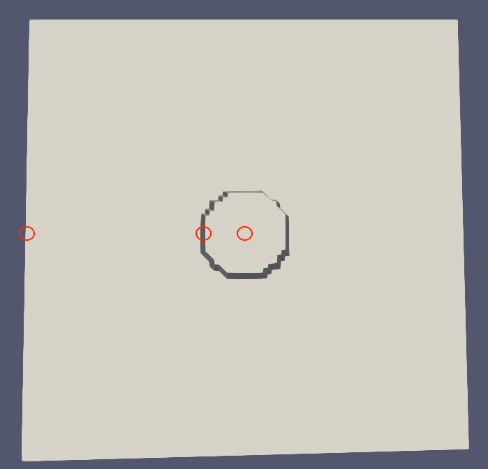
4.1.2 - Circular Dam Break
Since the momenta of this setup are always 0, we won’t mention them any further here.
The height however, is given by the following function:
tsunami_lab::t_real tsunami_lab::setups::CircularDamBreak2d::getHeight(t_real i_x,
                                                                       t_real i_y) const
{
    i_x-=50;
    i_y-=50;
    tsunami_lab::t_real sumOfSquares = i_x * i_x + i_y * i_y;
    return std::sqrt(sumOfSquares) < 10 ? 10 : 5;
}
We subtract 50 from both input parameters to realize the domain size of \([-50, 50]^2\) while using a simulation size of 100 and only positive numbers inside the main class.
Visualization
4.1.3 - Bathymetry and Visualization
We implemented a bathymetry reader to provide the bathymetry data using a csv file:
#dimensions
DIM,100,100
#x,y,bathymetry
40,30,30
41,30,30
42,30,30
43,30,30
44,30,30
45,30,30
46,30,30
47,30,30
48,30,30
49,30,30
50,30,30
51,30,30
52,30,30
53,30,30
54,30,30
55,30,30
56,30,30
57,30,30
58,30,30
59,30,30
This creates a wall which can be seen clearly in the following animation:
Note
The visualisation was created with ParaView using the TableToPoints and Delaunay2d filters.
The shown example can be replicated by running the project with the following configuration:
{
"solver": "fwave",
"nx": 50,
"ny": 50,
"simulationSizeX": 100,
"simulationSizeY": 100,
"setup":"CIRCULARDAMBREAK2D",
"bathymetry":"resources/bathymetry/singleWall2d_100x100.csv",
"hasBoundaryL": false,
"hasBoundaryR": false,
"hasBoundaryU": false,
"hasBoundaryD": false,
"endTime":20
}
Task 4.2 - Stations
4.2.1/2 - Station setup
Inside the config.json file we introduced a stations array where the user can provide multiple stations. The mandatory variables are: name, x-position and y-position.
e.g.
"stations":[
    { "name":"station_1", "locX":0, "locY":10 },
    { "name":"station_2", "locX":5, "locY":10 },
    { "name":"station_3", "locX":10, "locY":10 }
]
(File: Station.cpp)
Constructor
tsunami_lab::io::Station::Station(t_real i_x,
                                  t_real i_y,
                                  std::string i_name,
                                  tsunami_lab::patches::WavePropagation *i_waveProp)
{
    m_x = i_x;
    m_y = i_y;
    m_name = i_name;
    m_waveProp = i_waveProp;
    m_stride = i_waveProp->getStride();
    m_data = new std::vector<std::vector<t_real>>;
}
The constructor reiceives the position and name of the station and additionally the WavePropagation patch. We use the latter to access the simulation data.
capture()
void tsunami_lab::io::Station::capture(t_real i_time)
{
    std::vector<t_real> capturedData;
    capturedData.push_back(i_time);
    if (m_waveProp->getHeight() != nullptr)
        capturedData.push_back(m_waveProp->getHeight()[t_idx(m_x + m_y * m_stride)]);
    if (m_waveProp->getMomentumX() != nullptr)
        capturedData.push_back(m_waveProp->getMomentumX()[t_idx(m_x + m_y * m_stride)]);
    if (m_waveProp->getMomentumY() != nullptr)
        capturedData.push_back(m_waveProp->getMomentumY()[t_idx(m_x + m_y * m_stride)]);
    if (m_waveProp->getBathymetry() != nullptr)
        capturedData.push_back(m_waveProp->getBathymetry()[t_idx(m_x + m_y * m_stride)]);
    if (m_waveProp->getHeight() != nullptr && m_waveProp->getBathymetry() != nullptr)
        capturedData.push_back(m_waveProp->getHeight()[t_idx(m_x + m_y * m_stride)] +
                            m_waveProp->getBathymetry()[t_idx(m_x + m_y * m_stride)]);
    m_data->push_back(capturedData);
}
The capture function only receives the time as input and puts the values height, momentum X/Y and bathymetry into a captured data vector. In the end this vector gets pushed into the m_data vector which we created in the constructor.
write()
void tsunami_lab::io::Station::write()
{
    std::string l_path = m_filepath + "/" + m_name + ".csv";
    std::ofstream l_file;
    l_file.open(l_path);
    // write the CSV header
    l_file << "time";
    if (m_waveProp->getHeight() != nullptr)
        l_file << ",height";
    if (m_waveProp->getMomentumX() != nullptr)
        l_file << ",momentum_x";
    if (m_waveProp->getMomentumY() != nullptr)
        l_file << ",momentum_y";
    if (m_waveProp->getBathymetry() != nullptr)
        l_file << ",bathymetry";
    if (m_waveProp->getHeight() != nullptr && m_waveProp->getBathymetry() != nullptr)
        l_file << ",totalHeight";
    l_file << "\n";
    // write data
    for (std::vector<t_real> elem : *m_data)
    {
        for (t_idx i = 0; i < elem.size()-1; i++)
        {
            l_file << elem[i] << ",";
        }
        l_file << elem[elem.size()-1];
        l_file << "\n";
    }
    l_file.close();
}
The write function saves all captured data into a station-csv-file.
(File: main.cpp)
Inside the main function we introduce the l_stations vector and set it up with the following code:
if (l_configData.contains("stations"))
{
    for (json &elem : l_configData["stations"])
    {
        tsunami_lab::t_real l_x = elem.at("locX");
        tsunami_lab::t_real l_y = elem.at("locY");
        l_stations.push_back(new tsunami_lab::io::Station(l_x,
                                                          l_y,
                                                          elem.at("name"),
                                                          l_waveProp));
        std::cout << "Added station " << elem.at("name") << " at x: " << l_x << " and y: " << l_y << std::endl;
    }
}
...
if (l_simTime >= l_stationFrequency * l_captureCount)
{
    for (tsunami_lab::io::Station *l_s : l_stations)
    {
        l_s->capture(l_simTime);
    }
    ++l_captureCount;
}
    l_timeStep++;
    l_simTime += l_dt;
}
The stations output frequency determines how often the capture function for each station is called.
for (tsunami_lab::io::Station *l_s : l_stations)
{
    l_s->write();
}
Now the csv files are getting written.
4.2.3 - 1d vs 2d dambreak
The positions of the stations can be seen in the following images of the initial setups:
1d |
2d |
|---|---|
|
|
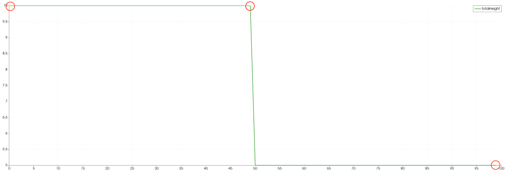
The following images show the water height in relation to the time at one particular position. Each station collected data with a frequency of 1 Hz.
1d |
2d |
|---|---|
|
|
|
|
|
|


Observation
In the 1d case the wave starts at height 10 and propagates to the right. There is a constant middle state around 7.2 meters. In the third image is shown that on the right side the height increases to the end.
In contrast, the height of the initial high water area decreases much faster in the 2d case. It also dips below the final height which is approximately 5 meters. The final height in the 2d case is lower than the one in the 1d case. Additionally, in picture 3 is the shockwave visible.